Effective Cartography
Mapping and Analysis with Categorical Data and SQL
There are two major families of GIS data models: Vector-Relational data models represent classes of things and conditions as rows in tables, each row being distinguished by a collection of attributes. Raster data models represent locations and conditions with cells that are like pixels in an image. This tutorial looks at the basic functions of Relational Databases, extended to handle vector data types. For more of the background on relational data models you can take a look at the Vector Relational Data Models page. This tutorial is also going to be an opportunity to talk about some of the ways that tables are encoded and exchanged -- topics that are discussed in more detail on our page about Data Formats for Geography.
In short, there is a standardized toolkit for using tables to store references to things and their attributes. This toolkit is called Relational Database Management Systems or RDBMS for short. If tables and their rows and columns are structured according to certain rules, then the RDBMS toolkit provides a set of functions (Structured Query L:anguage, or SQL) that makes it easy to explore relationships amongst the things and conditions represented in a table or in a system of tables. Functions of SQL include: Queries, Sorts, Summaries, and Joins. This tutorial will demonstrate some ways that we can employ these tools in ArcMap to perform logical experiments with relational data models. Perhaps we can even use tables of observations to learn new and useful things about the world!
Our purpose in exploring geographic data sets may be to discover useful distinctions and associations among things represented by data and then to portray these on a map. Most of the time, we will be using data that was collected for purposes different from ours. Quite often, the referencing schemes we find in data incorporate very fine categorical distinctions, most of which are irrelevant for our purposes. Because effective, credible communication requires us to be concise, it is usually the case, that we must transform complex category schemes to simpler ones, tailored to the distinctions that are important in our particular situation. This tutorial will examine some typical problems of using categorical referencing systems and to work some techniques for transforming one category scheme to another. This tutorial will take us through some of the fundamental principles and operations pertaining to tables and feature classes in ArcMap, including graphical, spatial, and attribute selections, and table joins.
Download the sample dataset
Download the State-Wide 1971-1999 Land Use Shape File and its Layer File
It happens that the MassGIS download for the state-wide land use layer does not include the .lyr file that contains the symbology and labels for the land use classes. Here is a link to a zip archive that includes the full state-wide 1971-1999 Land Use polygons with the .lyr file. This archive also includes the lookup table that is referred to later in this tutorial. If you just want to lookup table and the .lyr file, here is a zip file that just includes these
Workshop Outline
- Explore Land Use Data
- Discussing Areally and Semantically Categorized (Chunky) Data
- Explore Land Use Change Using Queries and Summaries
- Categorizing Data in Using a Layer's Symbology Properties
- Working with Legends in Layouts
- Fix Legend Headings
Display Tricks
Introducing Table Joins and Lookup Tables
- Joining A Lookup Table to a Feature Layer
- Explore a Look-Up Table
- Enjoy Easy Reclassification Using a Lookup Table
- Managing and Creating Categories with a Lookup Table
How to Create your Own Lookup Table
Video of this Tutorial!
- Part 1: Queries, Views, Sorts and Summaries
- Part 2: Table Joins -- Recategorizing Data with Lookup Tables
Explore the Land Use Data
For this demonstration we are going to look at a very interesting dataset from MassGIS that reflects land use change from 1971 to 1999. It is very important to understand the spatial and categorical granularity of these data so we can evaluate how well it suits our purposes. So read the metadata and explore the methodology by which the data were collected. The on-line metadata at the MassGIS web site may be easier to read. Especially examine what is said about the development of the 21 class land used coding scheme for 1971 and how it was extended to 37 classes in 1985. See how the code definitions are provided in the section of the metadata entitled, Land Use Code Definitions.
Awkward Lumpiness of Categorical Classification
Take a look at the description for the land use class, Urban Open. When this dataset was being developed, it seems that the distinction between parks, cemeteries and urban institutional campuses was not considered important. It is likely that for your purposes, (for example, understanding bird habitat) you might wish that you could have better control over this class. As it happens, you might be able to use another layer, for example Protected and Recreational Openspace may be useful, as it has many different categories, such as Prim_Purp (Primary Purpose that wil help you discriminate among many different sorts of open space.
Awkward Lumpiness in Aerial Units
Before using a dataset in a real decision-making situation, you should understand the spatial granularity of the data. For example, with the 1999 Land Use layer, the methodology included a rule that no polygons smaller than 1 Acre would be created. Obviously, this is going to lead to further generalization and omission of detaial, that might be important, depending on your specific purposes. When you look at the pattern of polygons that make up this exhaustive identification of Land Use, you can see that this characterization has a lumpiness both in terms of the semantic definitions of what "Land Use" can be, but also a granularity or lumpiness established by the method of observation.
Add the Land Use Data to ArcMap
- Use Windows explorer to look in the Sources\greenline_ext_massGIS_2018\landuse_1971_1999 folder. See that there is a shape-file and a layer file and also a file named lu21_lut_pbc.dbf
- Now in ArcMap, use the Add Data button to add the layer file, 37Landuse_Solid_Color.lyr to ArcMap
- Inspect the attribute table, and have a look at how the fields in the table correpond to the atribute definitions and land use codes inthe metadata.
Discussing Areally and Semantically Categorized Data
One of the biggest instinctive traps involved with discussing spatially and semantically categorized observations -- is to disregard and completely ignore the idea that there is any problem with lumpiness. Once you are aware of this problem hopefully you will understand that analysts who fail to mention this, are giving the impression that they are not aware that there is a problem. As an analyst yourself, even if you are aware of the problem you should not assume that your audience is immune from this trap.
The way out of this is simple. Consider the Things and Conditions expressed in your conceptual model. And the Spatial Mechaism by which your hypothetical things affect each other. Your conceptual description shuld be specific enough so that we understand the actual granularity of the way these things and conditions mesh in the real world. For example in the case of Bird Habitat, I should consult an avian ecologist who might tell me that the species of birds I am interested in requires patches of trees for nesting, and acertain amount of vegetation on the ground.
On the other hand, when we discuss data, such as land use data, we should keep in the forefront of the discussion, that while certain of the semantic classes may be helpful for distinguishing areas that may be more or less suitable for birds, yet on the other hand, we don't have information about actual clumps of trees. Rather, the Things reflected in the land use data are relatively large polygons of over an acre or more which are uniforml;y assigned to some generalized category. A good way to forefront this idea is to mention the issue of the minimum mapping unit (discussed above) explicitly in your text when you introduce the land use data.
The tricky part of the discussion is that the idea that the land use data is not perfect does not mean that it is utterly useless. (that would be too easy!) In the case of 1971 and 1985, this may be the best information that we have regarding some aspects of Bird Habitat that were observed at that time. What you must do is speak realistically about the specific of errors that you believe may result from the use of these data. Note that the same data-set might overestimate the existiance of a condition in one sort of place, and under-estimate the same condition in other areas. It is not enough to state that these errors may exist, you should point our specific types of important land use conditions that may be missed or falsely indicated with respect to your decision-making context.
Ultimately, this discussion will lead you to make useful recommendations for datasets that may do a better job of representing some aspects of the Things and Conditions that are of interest. -- for example, you might find betterdata about open spaces protected for the purposes of habitat preservations, wetlands data from the USGS.
Explore Land Use Change Using Queries and Summaries
Having our land use data organizes in a table allows us to filter the collection of polygons according to their attribute values to learn interesting things. IN the next demonstration, we will explore land use change from 1971 to 1999 using relational queries, or as they say in ArcMap, Select by Attributes.
References
Use Select By Attributes to Explore Industrial Land Use
- Right-Click the Land Use layer in your table of contents and choose Open Attribute Table
- Press the Select by Attributes button in the middle of the tool bar at the top of the table browser.
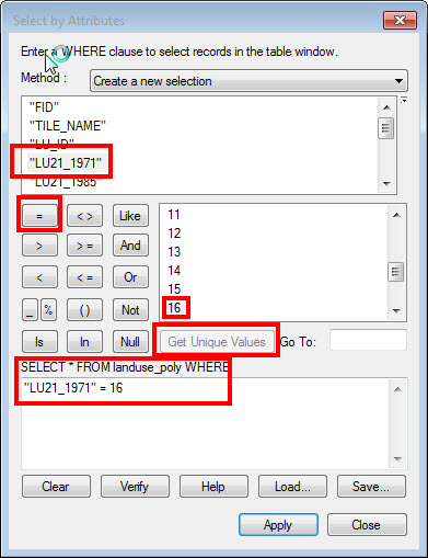
- Create a filter expression to select the polygons having a value for Lu21_1971 = 16 as shown in this screen shot
- Press Apply
- Take a look at the bottom of the table window, and notice that there are 241 out of 5926 polygons selected.
- Scroll up and down in the table window to find some selected rows.
- Press the Show Selected Records button at the bottom of the window to show only selected records. Don't forget to change this back to View All Records or next time you look at this table, no records wil show up!.
- Look at the map window, notice that the selected polygons are outlined in blue.
- Now, Right-Click on the column heading for Area_Acres and choose Statistics. ArcMap shows you a few statistical summaries for the selected records. The value for Sum is the total acres of the polygons that were coded as Industrial Land in 1971!
- Now, what if you wanted to see the polygons that had been coded as industrial in 1971, but had changed to some other land use in 1999? Hint: change your query expression to "LU21_1971" = 16 AND "LU21_1999" <> 16
Making queries in ArcMap is very powerful and there are many ways of doing it. A good way to learn about these is to click on the Help button at the bottom of the Select by Attributes Window.
Filter a Layer using a Definition Query
Using Select By Attributes to filter data is a useful way to explore. But what if we wanted to make a map that highlights just the polygons that had changed form Industrial land in 1971 to some other land Use in 1999? We can see those polygons on the map now, but they are all mixed up with the other land use polygons, and it is hard to find just the ones that we are interested in. A Definition Query is a layer property that allows us to restrict the polygons that are visible in a layer using an attribute query.
ReferencesSetting a Definition Query
- Double-Click on your Land Use layer in the table of contents to expose the layer's properties.
- Go to the Definition Query Tab in the layer properties.
- Click the Query Builder Button at the bottom of the Definition Query dialog.
- Build your query as we did above, or just cut and paste it form here: "LU21_1971" = 16 AND "LU21_1999" <> 16
- Click OK.
Notice that most of the polygons form the 1999 Land Use layer disappear. Our layer now shows only the 44 polygons that have changed form from Industrial in 1971 to some other value in 1999! This way of restricting layers according to queries can be very useful. It does not create any new data on our hard drive. So you could copy this to a new layer named Industrial Re-Use, 1971 - 1999 if you wanted to. For now lets just remove the definition query and proceed to explore some other techniques.
Removing a Definition Query
- Go back to your definition Query property of your Land Use 1999 layer.
- Select and delete the query expression
- Click OK.
- All of the 5926 polygons should re-appear.
Categorizing Data in Using a Layer's Symbology Properties
The ArcMap symbology editor is an easy way to apply symbols to features according to their attributes. Fro the purposes of making maps, the symbology editor can do three things for us:
- Let us apply symbols to features according to their attribute values
- Let us associate easy-to-understand labels to the legend categories
- Allow us to make more generel categories by grouping existing, finer-grained categories together.
In real life, we can come across category schemes that have hundreds of potential values. But to communicate ideas about land use concisely we will need to reduce the number of distinctions to highlight those that are critical for our study area and for our decision-making context. Cartographers generally agree that a concise legend should have no more than 7 or 8 color classes. We already know a couple of very effective ways of pruning needless categories from our legend.
Extract the land use polygons so that your shape file includes only those polygons that intersect with your map
There are likely many categories of land use that occur inth4e state-wide layer that do not occur in the limited area surrounding your area of interest. So once you desice on the scale and extent of your map, you can extract a new land use shape file using your trusty techniques that we learned in our tutorial on Organizing Data. Once you do this, you wil find that you have many fewer land use categories to deal with. If you stil have more landuse clsses that you want, and if some of the distinctions are not meaningful in yoru decision-making context, you can combine categories using he legend editor.
References
Extract your land use polygons covering your study area to a new shape file
- Use the zoom and pan tool to decide on a coverage for your new map. You may want to do this in layout mode.
- Right-click your land use layer and extract the polygons within the view extent to a new shape file. Be sure to save this to your project_data folder.
- Then you can make a copy of the original land use layer, by rigth clicking it and choosing Copy and then right cliking the data frame (the thing at the top of your table of contents that is named Layers and choose Paste Layers
- Rename this layer AOI Land Use where AOI is the name of your area of interest.
- Set the Source property of this layer to reference your new shape file.
This feature class (shape file) and its layer should now have a lagend that is much reduced in terms of the number laf land use categories. And these categories should all be represented withi your study area.
Use the Layer Symbology Properties to Consolidate Categories
Even though your legend has fewer categories, you may stil want to combine some of them to make your description of the setting more concice. To do that you can group categories in the Symbology properties of the layer as we did in the exercise on Nuts and Bolts of Mapping.
References
Remove Categories Using the Legend Editor
- Click the Plus Sign next to your new Land Use layer and look at the nice legend of 37 Land Use categories with nice labels.
- Right-Click your new land Use layer and choose Open Attribute Table to inspect the attributes of each polygon.
- Take a look at the data fields and their values. For example, see the values for Lu21_1999. Note how the values for Lu21_1999 correspond with the values listed in the Land Use Code Definitions in the MassGIS metadata for this layer.
- Note that the legend labels do not appear anywhere in our table! They are in the metadata.
- Double-Click the layer to go to its properties, and click the Symbology tab to look at how the layer is applying a Unique Values classification, using the values of LU37_1999. The values in this field are integers, but someone has added values to the Label field to associate human readable labels for each value of the code.
- Many of these land use categories don;t appear anywhere on the map. To see which these are, click the Count button at the top-right of the list of legend categories. You wil see the number of polygons that are in each class.
- Any category that has a count of zero can be removed by right-clicking it andchoosing remove.
Consolidating similar classes
Depending on your area of interest and your decvision-making question, you can fine-tune your land use categories to make a more concise presentation. Id the distinctioon between two classes of land use is of no interest to the decision-maker, you can group them together as described below.
Consolidate Similar Classes using the Legend Editor
This is a demonstration: the categories that you choos to consloidate for youtr project wil require some thought.
- Scroll down in the legend editor and find the legend entries for the values of 10, 11, 12, and 13. They are all different sorts of Residential.
- Control-Click to select all four of these residential classes, and then right-click and choose Group Values. We have just created a more general class land use class that lumps all of the Residential categories together into a class called 10;11;12;13
- Click on the Label value for the grouped values to change the name of this new legend entry to Residential.
- Click OK and you can admire your new, lumpier classification.
Un-Group Categories Using the Legend Editor
- Go back to the symbology properties for your Simplified 1999 Land Use layer.
- Find the legend entry for your grouped Residential classification, right-click it and choose Ungroup Values.
- Notice that the meaningful labels disappear. We would have to go back to the metadata to look these up.
Recategorizing data is a very common task in the world of GIS, because people who create data tend to use very fine-grained category schemes. Your aim should be to make a land use map that answers the questions that a a decision-maker might have regarfing your study area and your decision-making context. As a general rule you don't want to have more than 8 categories. Doing a good job with this requires you to look at the metadata to understand what the existing categories mean, and it will also requires that you think about the general land-uses that cover the context of your study area and the specific land uses that may be most important in terms of the things and conditions and spatial relationships that you are concerned with. You don't want to confuse people with a lot of distinctions that are irrelevant. On the other hand, you also shouldn't use categories that are too broad -- because this can make it look like you are deliberately hiding, or unwittingly disregarding something. So picking land use categories is a balancing act.
Use Conventional Land Use Shades
The reason that we are going through all of this trouble to recategorize data is so that we can describe the critical aspects of a situation concisely and efficiently. We want to streamline the process of understanding these things for our clients and the general public. It is also true that in the process of working through this. we are also going to inform ourselves, and will probably also see how we can reformulate our question to make better use of the information that we have. One very important part of communicating concisely is touse the conventional shading scheme for land use categories that is discussed on the page, Elements of Cartographic Style.
Working with Legends in ArcMap
Thematic maps portray data using a vocabulary of symbols. The legend on a thematic map is one of the first places that a map user will look when trying to figure out what the map is about. It is relatively easy to insert a legend on your map layout, but there are some important aspects of preparing your legend that may not be obvious.
All Legend Classes should Appear on the Map
A good thematic legend should not include more than eight classes. Beyond this number it becomes a challenge to discriminate the meaningful distinctions. Usually these distinctions are part of the argument that you are making with your map. Considering this, it is not a good idea to show categories in your legend that do not appear in the map.
Resources
- Go to View > Layout View
- Organize your layour sothat there is room for a legend on your map.
- Go to Insert Legend which wil expose the Legend Wizard.
- The first panel of the legend wizard opens with lots of layers in the legend. You can use the << button to clear the legend.
- Then you can use the > button to add your land use, and your Open Space layers. Then press Next
- In the next dialog box you can get rid of the heading that says "Legend."
- I normally just take the defaults for the rest of the inmitial legend set up.
At this point you have a legend, but it usually has too many items in it. In the next stage, you can reduce the number of items toinclude just those that apper on your map.
Reducing the number of Items in your Legend
- Use the black arrow Select Elements tool to double-click your legend in the layout. This wil expose alegend properties dialog.
- Go to theItems tab.
- Check the option: Only Show classes that appear in map extent
- Then you can click OK
Fixing Legend Headings and Labels
By default, the legend heading wil be the name of the field that the categorical symbolization is based on. Inmost cases this field name will not be meaningful to the average person. You also may have a legend category for All other Items You will want to change this. The following steps discuss how to do this.
Resources
Fix Headings and Legend Labels in the Table of Contents
- IN the ArcMap table of contents, you can press on your legend heading. Mine was called BirdHab. Pressing on this with the left mouse button wil allow you to type in a new name -- Like For example: Reclassified 1999 Land Use
- If you want to change any of the individual legend labels, you can also changhe these in the table of contents.
- Notice that the changes that you make in the table of contents are automatically reflected in your layout legend!
Getting Rid of the All Other Values item
- Double-clidk your reclassified land use layer to expose the Layer Properties
- In the Symbology properties, notice that you can un-check the box next to All Other Values
Using Transparency and an Aerial Photo
The spatial and categorical lumpiness of our land use data most definitely pose a problem for many applications where knowing the actual land use is important. There are definitely questions for which this data-set can provide useful answers. But in any analytical context, the methodology and the categorical and spatial lumpiness needs tobe discussed,. If it is not, then the analyst is implying that the data are perfect.
One very evocative way of calling attention to the complexity of the real-world patterns is to make your land use and open-space layers transparent, and show them on top of an Aerial photo. Changing the transparency of a layer can be done by simply tweaking the Transparency parameter in the Display Properties of the layer. Simple enough; but the problem is that if you have two layers, like Open-Space and 1999 Land Use, you will find that the Transparency (or Opacity...) of two layers adds up. So that the aerial will be more difficult to see in areas where Parks are over-layed on Land Use. To fix this, you can create a group layer for transparent layers, put your parks and land use data into it, and adjust the transparency of the group. Of course your Aerial photo would be underneath.
References
Some Examples of Effective Graphical Hierarchy with Land-Use-Tinted Aerioal Photography
Manage Transparency of Multiple Layers with a Group Layer
- Create a new group layer. You could name it Transparent Layers the name doesn't matter.
- Drag in the l;ayers that you want to treat transparently, like Land Use and Protected Open-Space.
- Check the Display Properties transparency of the individual layers. They should all be completely opaque (0 Transparency.)
- Open the Display properties of your group layer and experiment with the transparency. Hint, setting transparency to 90 makes thelayer very transparent. Setting it to 10 makes the layer very opaque.
Note that these topics are not required for your categorical data exercise!
Part 2: Introducing Table Joins and Lookup Tables
The process of recategorization may require several trials and adjustments. Using the arcmap legend editor to group categories as demonstrated above may not be too difficult when you have only 35 categories, but this is quite aggravating if you have datasets that include hundreds of distinct values. This is why professional data wranglers use a powerful relational database techniques called Table Joins and Lookup Tables to manage categorical data.A Lookup Table is a table that translates a complex set of categorical codes (like our MassGIS Land Use codes). to one or more generalzed categorical Schemes.
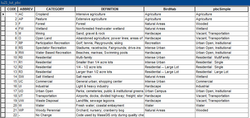
Notice how the table pictured above has a row for each of the MassGIS Lu_21_ land use codes. And for each code there are four different categories applied. The most diverse class is carried in the Definition column. There is a more general classification given in the column named Category in which all four Residential codes are lumped together into a common class. Another column, BirdHab shows a classification of land use that was developed for the purposes of evaluating land use from the perspective of a person interested in bird habitat.
Joining A Lookup Table to a Feature Layer
The names for the alternate land use classifications that appear in the columns of our lookup table would be very useful if they were columns in the attribute table of the MassGIS Land Use layer. If they were, we could apply the categorization using the legend editor in the layer's symbology properties. We can accomplish this using a technique known as a Table Join.
References
- An Overview of Tables
- Adding Tables in ArcGIS
- Using the ArcMap table of Contents
- Common Tables and Attribute Tasks
Open and Inspect A Lookup Table
- Use your Add Data button to add the table sources/greenline_ext_massgis_2018/land_use_1971_1999/lu21_lut_pbc.dbf Note that when you open a table in ArcMap, your Table of Contents shifts to List by Source mode. Your table of contents wil not show you plain tables when you are in the ordinary list by Drawing Order mode.
- Right-Click lu21_lut_pbc and choose Open
- Take a look at our lookup table. Notice that it has a row for each of the 21 land use codes. For each of the 21 classes, our table has alternative classifications which are more general. For example, you can see that in the data field (column) headed, Definition there are four different classes of Residential land use, corresponding with codes, 10, 11, 12, and 13. The data field, Category classifies all of these into a single more general category, Residential.
Investigate How the Land Use Attribute Table References Rows in the Lu_21_lut_pbc Lookup Table
- Right-Click your Simplified Land Use Layer in the Table of Contents and open its attribute table.
- You now should have two tables open in the ArcMap table window. You can switch back and forth between them by clicking the little tabs at the bottom-left of the window.
- In the Attribute table for your Simplified Land Use layer, notice how there is a row for each of the 5926 polygons.
- The column, Lu21_1999 has a value for each polygon that identifies its 1999 land use, using the 21-class coding scheme.
- For any one of those LU21_1999 values you can look up the associated row in the Lu_21_lut_pbc lookup table having the same value in the column, Code.
- In the language of relational databases, we say that Code is the Unique Key in the lookup table, and LU21_1999 is the Foreign Key in the feature attribute table.
- To find the associated general and more specific classifications for any polygon, we can look up the category values in the Lu21_lut_pbc lookup table.
Hopefully that idea of how the attributes for rows in one table can reference rows in a lookup table makes sense. Because it turns out that we can automate this process with a procedure known as a Table Join
References
Joining your Lookup Table
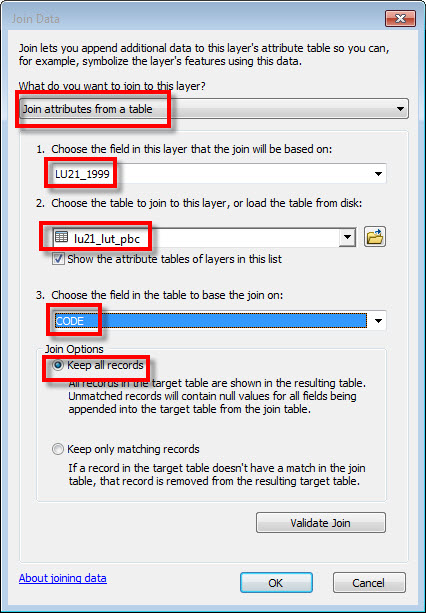
- Right-Click your Simplified 1999 Land Use layer in the ArcMap table of Contents and choose Joins > Join to expose the Join Dialog Box.
- Identify the table you wish to Join and the appropriate linking fields as shown in this screen shot.
- Click OK.
- ArcMap may show you a reccomendation that you index the key field in your table. Click Yes.
- Now, look at the attribute table for your Simplified 1999 Land Use layer.
- Scroll to the right and notice that each polygon now has values for the classifications from the lookup Table!
This table join is a virtual view of the two tables joined togethr which is part of the Simplified 1999 Land Use Layer but it has changed nothing about the original shape file on the disk. To see this you could look at the attribute table of the original Land Use (1999 37 Classes) layer and see that it is not joined.
Enjoy the Easy Reclassification and Labeling of your Legend
Joining tables can be a little confusing and intimidating at first, but the next step will show you why it is worth it. We will go back into the properties of our new Simplified 1999 Land Use Layer, and see how easy it is to create a new legend based on any of the land use classifications in the lookup table.
References
A New Legend
- Double-Click on your Simplified 1999 Land Use Layer to expose its properties.
- Click the Symbology Tab
- Now, pull down the Value Field tab and scroll to the bottom of the list of columns. You wil see the new columns form the table join. You now can choose to classify your land use polygons accodeing to the pbc_simple classification try it!
- The legend labels now fill themselves in automatically!
Managing Categories in the Lookup Table
You see how the lookup table has made the application of categories fairly easy. The next step should make it clear how to use the lookup table to adjust and manage classes. In map making, you never get things right the first time. Adjustments are always necessary at some point. In our case, once we look at the map, we can see that we have too many categories. The distinction between wetlands and woodlands is not necessary in our case. So we need to create an even simpler classification. To fix this we will create a new column in our lookup table to hold a new version of our pbcSimple classification. Then we can edit a few of these values to create an even simpler scheme. Finally we will re-join the lookup table and apply the new, even simpler scheme.
References
Creating a New Classification in our Look-Up Table
- Find our Lu21_lut_pbc.dbf lookup table near the bottom of your ArcMap table of contents. You may need to change the table of contents back to list by Source mode.
- Right-click the table and choose Open so you can view it in the Table window.
- Pull down the Table Options pull down at the upper left corner of the Table window and choose Add Field.
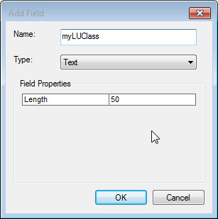
- Create a new field named myClass. Make sure to choose Type: Text. See screen-capture.
Now that you have a new field, there are a few different ways of setting its values. In the next several sterps we will explore some of the ways of doing this. First we can set all the values based on the values of another field in the table. After that, we can select a specific row oe rows and set their values.
Setting All of the Values for a Field based on the Values of Another Field
- You should begin this step with the Lu21_lut_pbc.dbf table open and no rows selected.
- If you have any rows selected, you should un-select them with the Clear Selection button at the top of the Table window.
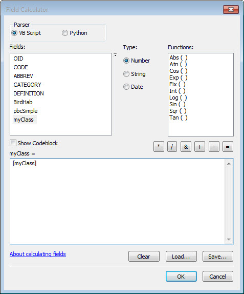
- Now right-click the heading of your new myClass field and choose Field Calculator.
- In the field Calculator dialog, find the pbcSimple field in the Fields list, and double-click it.
- This will cause the name of the field to appear in lower panel as shown in this screen shot.
- Press OK in the field Calculator and you wil see that al lof the values of MyClass have been calculated to be the same as the values of pbcSimple.
Setting the Values for Selected Records
- Note that this operation does not work correctly if you are in View Layout mode. Make sure that you use the View menu and choose Data View
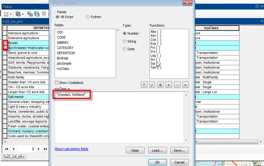
- with theLu21_lut_pbc.dbf table open, select one or more rows in the table by clicking in the little white box at the very left side of a row. Control-click to select several rows. I suggest that you click the rows for Codes 3,4,14 and 21, for Forest, Wetland, Salt Wetland, and Woody Perennial. In our new class system, we want all of these to be in a new class called Wooded and Wetland.
- Now right-click the heading of your new myClass field and choose Field Calculator.
- In the field Calculator dialog, clear out the bottom panel to remove the reference to the [pbcSimple] field if necessary.
- Now type "Wooded and Wetland" into the lower panel - including quotes as shown in This screenshot
- Press OK in the field Calculator and you will see that the values of MyClass have been calculated for just the selected rows!
Now that you have modified the lookup table to add your own classification scheme, you can use it to create a new legend. But before you do, you have to un-join the lookup table from the Simplified Land Use 1999 layer and join it again. Otherwise, your new column does not show up in as one of the choices in your Val;ue Field pull-down menu.
References
Removing a Join
- Right Click your Simplified 1999 Land Use layer, and choose Joins > Remove Joins > Remove All Joins
- Now add the join again as you did earlier See screen shot.
You now have a mastery of using lookup tables to manage categories! You now can assign appropriate land use symbols to your legend classes according to the conventions for land use shading discussed on the page Elements of Cartographic Style.
Creating Lookup Tables
The topics below cover one way of creating a lookup table for yourself using Microsoft Excel. These steps are not necessary for completing the homework for Fundamentals of GIS. Nevertheless, the techniques of passing tables in between Excel, ArcMap and dbf format are good to know if you need to create your own lookup tables. Another way of creating a lookup table is covered in the ArcMap on-line help topic Summarizing a Table before Joininig it.
Resources- Creating New Tables especially see "from text Files"
- About Working with Excel Tables in ArcGIS
Some Notes on Exchanging Tables between Excel and ArcMap
- The most flexible way of dealing with tables in ArcMap is the Dbase (.dbf) format. This format can be read and written by OpenOffice. Excel can read dbf, but won't write to it in the latest version.
- ArcMap can open Excel's .xlsx format directly, but these tables cannot be modified when they are open in ArcMap. So if you create tables in Excel, it is best to convert them to DBF right away by right-clicking them in the ArcMap table of contents and choosing Data Export Data. Note you must choose Save as type: dBase Table in the export dialog
- A DBase table cannot have more than 9 characters in its field names, nor can these names contain spaces or special characters that aren't simple letters, numbers and underbar characters. Nor can a field name begin with a numeral. So keep this in mind if you are creating tables in excel.
- Another gotcha of using excel with ArcMap is that sometimes ArcMap won;t let you use a table if it is open in Excel and Vice Versa. A good way around these problems is to use Excel to create new versions of tables, and export them as CSV. When you want to edit a table in Excel, create a new version.
- A Comma-delimited text file (.csv) is an easy way to encode and exchange information between programs, although some semantic information about data types, such as dates and numbers can get lost in the translation.
- The problem of data types not being discriminated in text files emerges most often when data values consist of numerals but are actually character strings (like zip codes.) In this case, leading zeros are chopped off, and can sometimes be difficult to add back on.
- You can also save tables in an ArcGIS Geodatabase. This format has fewer restrictions on field names, etc, but is less portable. For example it can't be opened in Excel.
Create a Lookup Table in Excel from the MassGIS Metadata
- Explore the Data Dictionary for the 21 Class land use code from the Land Use metadata.
- Consider how you might use the legend editor to reclassify these codes into a concise categorization that emphasizes the distinctions that are critical for our question.
- Copy and paste the data dictionary from the metadata into excel. Today we are lucky because we can paste this into excel and it simply fills in rows and columns of a table that requires few modifications. Often making a lookup table is more of a headache than this. Note: THis trickworks from the metadata web page, but not the PDF version!
- Save your excel spreadsheet as an .xlsx file in your Project_Data folder.
Open Excel Table in ArcMap and Save it as a DBF
- Use the Add Data button to add the excel table in ArcMap. Note that you have to double-click the excel icon in the add data dialog to see the various worksheets in the excel table.
- While ArcMap can open an excel table, it can't alter them, and often does not register updates that you make in Excel. It is best to export the table in DBF format and add this table to ArcMap before going further.
- Right-Click your lookup tabel in the ArcMap table of Contents, and choose Data > Export and click the little Folder Icon to enter the Save As dialog.
- Save your lookup table as Type: DBase. Make sure you save this to a location in your project folder that you will be able to find again.
- Now you can open your new table in ArcMap.
Advantage of DBase Format in ArcMap
Now that your lookup table is in Dbase format, you can add columns and change the values of data fields within ArcMap. While it may seem easier to do these things in Excel, the trouble is that ArcMap does not always see the changes that you make in Excel, and it is tricky to keep saving the Exel document and re-opening it in ArcMap if you wnt to make adjustments.
